

In 1952 Harry Markowitz published a 14 page paper in the Journal of Finance. It later earned him a share of the 1990 Nobel Prize in economics. The idea fits in one line: what matters for a portfolio is not how risky each holding is, but how the holdings move against each other. Diversification is not owning many things. It is owning things that do not all fall on the same day.
I learned this the expensive way. Early in my career I spent my energy on which stocks to own and almost none on how they combined. After many years of running systematic books, I would put it bluntly: the way you combine positions decides your drawdown more than the positions themselves. Here is the theory behind that, with the parts that break on Indian data marked clearly.
The core insight: correlation and diversification
Take two stocks. Stock A is expected to return 15% a year with 20% volatility. Stock B has the same 15% and the same 20%. Put half your money in each. The expected return is 15% whatever you do. The risk depends on one number, the correlation between them, written ρ (rho).
- If A and B are perfectly correlated (ρ = +1), portfolio volatility stays at 20%. Combining them bought you nothing.
- If they are uncorrelated (ρ = 0), portfolio volatility falls to about 14.1%. Same return, roughly 30% less risk.
- If they are perfectly negatively correlated (ρ = −1), volatility is 0%. Each move cancels the other. Two real stocks never behave like this, but it shows where the benefit comes from.
Put that in rupees. On ₹10 lakh, a one standard deviation bad year for a single stock at 20% volatility is a ₹2 lakh hit. For the uncorrelated pair it is about ₹1.41 lakh. You gave up no expected return to save that ₹59,000 of typical pain. That is why diversification is called the only free lunch in finance.
How many stocks is enough?
Extend the same maths to an equal weight portfolio of N stocks, each with the same volatility σ and the same average correlation ρ with each other. Portfolio volatility becomes σ × √(ρ + (1 − ρ) / N). Two things fall out of that formula. Adding stocks helps fast at first and then barely at all. And no number of stocks takes you below σ × √ρ, because the shared, market wide part of the risk never diversifies away.
- 1 stock30.0%
- 5 stocks19.9%
- 10 stocks18.2%
- 20 stocks17.4%
- 50 stocks16.8%
- Unlimited, the floor16.4%
Portfolio volatility, equal weight, from σ × √(ρ + (1 − ρ) / N) with each stock at 30% volatility and average correlation 0.3. Illustration, not a back test.
Read the table twice. Going from 1 stock to 10 removes 39% of the risk. Going from 20 to 50 removes another 2 points. Past about 20 names, more stocks mostly buys you more paperwork. If you want the risk lower still, you need something with a lower correlation, not more of the same thing.
The efficient frontier
Markowitz showed that for any set of assets there is a curve of portfolios that give the highest expected return for each level of risk. That curve is the efficient frontier. A portfolio on it cannot earn more without taking more risk, and cannot cut risk without giving up some return.
A portfolio below the curve is leaving something on the table. The same risk could have earned more, or the same return could have come with less risk, simply by combining the holdings differently. In practice almost every real portfolio sits somewhat below the curve, because the curve is drawn from estimates and the estimates are wrong. More on that below.
For factor investors the frontier idea becomes factor diversification. Momentum and value have historically had low, sometimes negative, correlation with each other. Two moderately good factors with low correlation can beat one excellent factor on a risk adjusted basis, for exactly the reason in the two stock example.
What MPT gets right
What MPT gets wrong: the practical limitations
The practical lesson: keep MPT's way of thinking, in correlations and diversification, but do not feed historical averages into an optimiser and trust the weights it prints. The inputs are too noisy. Simple, robust weighting such as equal weight or inverse volatility, which needs no forecast of expected returns, has held up better out of sample. DeMiguel, Garlappi and Uppal (2009) tested 14 optimised models against plain 1/N on seven data sets, and none beat 1/N consistently.
A worked example: blending two real sleeves
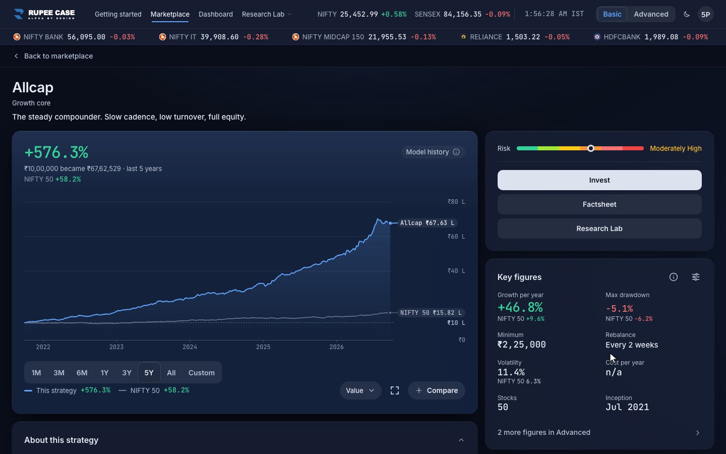
Here is the two asset formula with numbers from this site. The Allcap strategy's factsheet shows annual volatility of 23.58% for the model and 14.15% for the Nifty 50 over the same five year window. Suppose you split ₹10 lakh evenly between a Nifty 50 index fund and the Allcap model.
| Correlation you assume | Volatility of the 50/50 blend | Weighted average of the two | Benefit |
|---|---|---|---|
| 0.8 | 18.0% | 18.9% | 0.9 points |
| 0.5 | 16.5% | 18.9% | 2.4 points |
| 0.0 | 13.7% | 18.9% | 5.1 points |
Volatilities from the Allcap factsheet: model, back tested, weekly figures over rolling 5 years to 13 Jul 2026. Correlations are assumptions for the illustration.
Two Indian equity sleeves, one large cap and one all cap momentum, usually correlate strongly, so the honest row is the first one. You get under a point of risk reduction. The rows below it show what a genuinely different asset could do. That is why the multi asset strategies on RupeeCase add debt and gold sleeves rather than more equity names: the low correlation is the point.
What actually matters for systematic portfolio construction
From years of building systematic strategies, these are the MPT derived rules I still use:
- Diversify across factors, not only across stocks. Thirty momentum stocks diversify less than fifteen momentum plus fifteen quality stocks, because the factors correlate less than the stocks inside one factor.
- Correlation beats brilliance. Two decent, low correlation return streams usually beat one great one on a risk adjusted basis.
- Cap the sector bet. A momentum screen can quietly end up with half its names in one sector. A sector limit costs little return and removes a hidden single bet.
- Size by risk when volatility varies a lot. Giving less weight to very volatile names stops a few of them from driving the whole portfolio. Module 4.2 works through this with numbers.
Why MPT under delivers on Indian data specifically
Markowitz worked with assumptions that suit deep, liquid markets with fairly steady correlations. Indian equities break a few of them, which is why a naive optimiser often produces a portfolio that looks elegant in the spreadsheet and behaves badly in your demat.
Correlation regimes shift. In normal months large caps and mid caps move together only partly. When foreign investors sell hard, the correlation jumps and the benefit you optimised for shrinks. Use correlations from stress periods, or a blend of stress and normal, when you decide an allocation, not the full history average.
Impact cost is lopsided. The frontier ignores the cost of getting in and out. Trading a Nifty 50 name at sensible size costs a fraction of what the same rupee trade costs in a thinly traded small cap. NSE publishes impact cost for index constituents, and the gap between the two ends of the market is large. An optimiser handed the whole Nifty 500 will happily overweight small caps with great back tested returns, and the trades needed to hold those weights then eat the edge. A liquidity floor fixes this: exclude anything you cannot trade at your size without moving the price.
Foreign ownership links unrelated stocks. Many large caps have heavy foreign institutional ownership. A US rate move or a weak rupee can pull money out of that whole basket at once, so stocks from different sectors fall together. A sector view misses this. The quarterly shareholding pattern filed with NSE and BSE shows who owns what.
Factor returns swing hard. Indian factor returns have had long, sharp cycles. An optimiser fitted on a trailing window overweights whatever just worked and underweights whatever is mid drawdown. Equal weight blending, or a slow regime overlay, is the more robust answer even though it looks less clever on paper.
The conclusion is not that MPT is wrong. The core idea stands. The inputs and the constraints must match the market you trade.
Common mistake: counting names instead of correlations
The mistake I see most often is a portfolio of 25 stocks that is really three bets. Eight private banks and NBFCs, seven IT services names, ten stocks from the same capital goods theme. It feels diversified because the list is long. On a day when rates move or the rupee weakens, it trades like three stocks.
- Banks and NBFCs, 8 names32%
- IT services, 7 names28%
- Capital goods theme, 1040%
Illustrative equal weight portfolio, grouped by what drives each stock.
The check takes five minutes. Group your holdings by what actually drives them: interest rates, US technology budgets, government capex, commodity prices. If one driver explains more than a third of your money, you own a concentrated portfolio with a long list of names. Fix the driver exposure, not the stock count.
MythThe more stocks you own, the safer you are.
FactBeyond about 20 names the risk barely falls, and stocks that share one driver fall together. Lower correlation, not a longer list, is what reduces risk.
How this shows up in RupeeCase
Each RupeeCase strategy is a published rule: rank a universe by a momentum composite, hold the top names equal weighted, and rebalance on a fixed calendar. The holdings count is part of the design, from 5 names in the most concentrated strategy to 50 in Allcap. The multi asset strategies, such as Allcap Multi Asset, add debt and gold sleeves for the correlation benefit described above. Every factsheet shows the model's volatility, Sharpe, Sortino and maximum drawdown next to the Nifty 50, so you can see what the diversification bought. Line any two up on the compare page. All strategy figures are model, back tested.
Questions readers ask
Is Modern Portfolio Theory still used by professionals?
The ideas are used everywhere: correlation, diversification, the risk and return trade off. The raw optimiser fed with historical averages is used far less. Most practitioners constrain it heavily or replace it with simpler weighting that does not need return forecasts.
How many stocks do I need to be diversified in India?
With the formula above, most of the stock specific risk is gone by 15 to 20 names, provided they are not all driven by the same thing. Fifty names from one sector are less diversified than twenty from different sectors and factors.
Does diversification reduce returns?
It does not reduce expected return; the expected return of a mix is the weighted average of its parts. What it removes is the chance that one holding makes your year, and the chance that one holding ruins it.